Object Detection

See also: object classification

Template Matching

Linear filtering is also known as template matching. Convolution/correlation can be thought of as comparing a template (the kernel) with each section of the image.

• Consider the filter and image section as vectors
• Applying the filter can be interpreted as computing the dot product between the filter and the local image patch

The correlation is then normalized to between -1 and 1 using cosine similarity, where 1 is the value when the filter and image region are identical. This process is essentially finding the cosine similarity between template and local image neighbourhood

$\cos \theta =\frac{a\cdot b}{|a||b|}=\frac{a\cdot b}{\sqrt{(a\cdot a)(b\cdot b)}}=\frac{a}{|a|}\frac{b}{|b|}$

Then, we can map over the image and create a correlation map. Thresholding this gives us detections.

Good:

1. Robust against noise
2. Relatively easy to compute Bad:
3. Scaling (we can address this using scaled representations like a Gaussian image pyramid)
4. Rotation
5. Lighting conditions
6. Sensitive to viewing direction and pose (in 3D worlds)

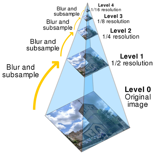
Gaussian Image Pyramid

Collection of representations of an image. Typically, each layer of the pyramid is half the width and half the height of the previous layer. In the Gaussian version, each layer is smoothed by a Gaussian then resampled to get the next layer.

Details get smoothed out (are completely lost) as we move to higher levels, only large uniform regions of colours in the original image are left.

Laplacian Pyramid

To do this, create a Gaussian pyramid and take the difference between one pyramid level and the next after smoothing but before subsampling.

At each level, retain the residuals (difference between smoothed image and normal image) instead of the blurred images themselves.

Constructing the pyramid, we repeat until min resolution reached:

1. Blur
2. Compute Residual
3. Subsample

Reconstructing, we repeat until original resolution reached:

1. Upsample
2. Blur
3. Sum with residual

Local Feature Detection

Moving from global template matching to local template matching (e.g.edges and corners)

As differentiation is linear and shift invariant, we can implement it as a convolution.

The discrete approximation is $\frac{\partial f}{\partial x}\approx \frac{F(X+\Delta x,y)-F(x,y)}{\Delta x}$ where $\Delta x$ is usually $1$. This is equivalent to a convolution $F$ is a $1\times 2$ filter with the first element is $-1$ and the second element is $1$. Note that the derivatives go up for the Y direction and the right for the X direction.

We usually smooth the image prior to derivative estimation. Increased smoothing

• eliminates noise edges
• makes edges smoother and thicker
• removes fine detail

Weights of a filter for differentiation should sum to 0 as a constant image should have derivative 0.

Edge Detection

The goal here is to identify sudden changes in image brightness as this encodes the vast majority of shape information.

An edge is a location with high gradient.

Mainly caused by

• Depth discontinuity
• Surface orientation discontinuity
• Reflectance discontinuity (e.g. change in material)
• Illumination discontinuity (e.g. shadows)

As we usually smooth prior to derivative calculation and convolution is associative, we can combine both steps and use derivatives of Gaussian filters.

$D\otimes (G\otimes I(X,Y))=(D\otimes G)\otimes I(X,Y)$

Sobel (Gradient Magnitude)

Let $I(X,Y)$ be an image. Then, we let $I_x(X,Y)$ and $I_y(X,Y)$ be estimates of the partial derivatives in the $x$ and $y$ directions, respectively. Then, the vector $[I_x,I_y]$ or $\nabla f=[\frac{\partial f}{\partial x},\frac{\partial f}{\partial y}]$ is the gradient and $\sqrt{I_x^2+I_y^2}$ is the gradient magnitude.

The gradient points in the direction of most rapid increase of intensity. The direction is then $\theta =\arctan \frac{\frac{\partial f}{\partial y}}{\frac{\partial f}{\partial x}}$. The strength of the edge is then the magnitude $||\nabla f||=\sqrt{{\frac{\partial f}{\partial x}}^2+{\frac{\partial f}{\partial y}}^2}$.

Marr/Hildreth (Laplacian of Gaussian)

Design Criteria

1. localization of space (find where the edge is)
2. localization in frequency (identify high frequency and low frequency edges)
3. rotationally invariant (rotation shouldn’t affect edges)

Find the zero-crossings (intercepts) of the Laplacian of the Gaussian. This is ${\nabla }^{2}G(x,y)=\frac{-1}{2\pi {\sigma }^4}[2-\frac{x^2+y^2}{{\sigma }^2}]\exp (-\frac{x^2+y^2}{2{\sigma }^2})=0$

Alternatively, we can say that subtracting the delta function from the Gaussian gives you an approximation of the Laplacian

Canny (Local Extrema of 1st deriv)

Design Criteria

1. good detection (reduce missed edges, reduced edges where edges don’t exist)
2. good localization (accurate edge detection)
3. one (single) response to a given edge

Find the local extrema of a first derivative operator.

Steps

1. Apply directional derivatives of Gaussian

2. Computer gradient magnitude and gradient direction

3. Perform non-max suppression Non-max suppression allows us to suppress near-by similar detections to obtain one “true” result. In images, we select the maximum point across the width of the edge (following the direction of the gradient).

   In implementations, the value at a pixel $q$ must be larger than its interpolated values at $p$ (the next pixel in the direction of the gradient) and $r$ (the previous pixel in the direction of the gradient). Interpolate as needed.

4. Linking and thresholding Trying to fix broken edge chains by linking separate edge pixels through taking the normal of the gradient and linking it if the nearest interpolated pixel is also an edge pixel. Accept all edges over low threshold that are connect to an edge over high threshold.

Author	Approach	Detection	Localization	Single Resp	Limitations
Sobel	Gradient Magnitude Threshold	Good	Poor	Poor	Thick edges
Marr/Hildreth	Zero-crossings of 2nd Derivative	Good	Good	Good	Smooths Corners
Canny	Local extrema of 1st Derivative	Best	Good	Good

Boundary Detection

How closely do image edges correspond to boundaries that humans perceive to be salient or significant?

One approach is using circular windows of radii $r$ at each pixel $(x,y)$ cut in half by a line that bisects the circle in half. Then, compare visual features on both sides of the cut and if the features are statistically different, then the cut line probably corresponds to a boundary.

For statistical significance:

1. Compute non-parametric distribution (histogram) for left side
2. Compute non-parametric distribution (histogram) for right side
3. Compare two histograms, on left and right side, using statistical test

Example features include

• Raw Intensity
• Orientation Energy
• Brightness Gradient
• Color Gradient
• Texture gradient

For this implementation, we consider 8 discrete orientations ($\theta$) and 3 scales ($r$)

Features

Corners are locally distinct 2D image features that (hopefully) correspond to a distinct position on a 3D object of interest in the scene.

Cannot be an edge as estimation of a location along an edge is close to impossible (the aperture problem)

Autocorrelation

Correlation of the image (distribution of pixel values) with itself. At each pixel, compute its partial derivative w.r.t. either the $x$ or the $y$ axis, $I_y=\frac{\partial I}{\partial y},I_x=\frac{\partial I}{\partial x}$.

Windows on an edge will have autocorrelation that falls of slowly in the direction of the edge but rapidly orthogonal to the edgge. Windows on a corder will have autocorrelation that falls off rapidly in all directions.

Harris Corner Detection

As a stats reminder, covariance is the direction of the correlation. The closer the covariance is to 1, the closer it is to a perfect positive correlation. -1 implies perfect negative correlation.

When drawing distrubtion, draw normals to edges going from low values (dark) to high values (white).

1. Compute image gradients over small region
2. Compute covariance matrix $\left[\begin{array}{cc}{\sum }_{p\in P}{I}_x{I}_x& {\sum }_{p\in P}{I}_x{I}_y\\ {\sum }_{p\in P}{I}_y{I}_x& {\sum }_{p\in P}{I}_y{I}_y\end{array}\right]$ (essentially fitting a quadratic to the gradients over the small image patch $P$)
3. Computer eigenvectors and eigenvalues of the covariance matrix.
4. Use threshold on eigenvalues to detect corners ($>0$ is a corner)

We can visualize the covariance matrix $C$ as an ellipse whose axis lengths are determined by the eigenvalues and orientation determined by $R$ (the rotation matrix). It tells us the dispersion of the gradients nearby.

As $C$ is symmetric, we have the covariance matrix as the ellipse equation

$f(x,y)=\left[\begin{array}{cc}x& y\end{array}\right]\left[\begin{array}{cc}1& 0\\ 0& 1\end{array}\right]\left[\begin{array}{c}x\\ y\end{array}\right]=\text{const}$

Where the minor axis is ${\lambda }_{max}^{-1/2}$ and the major axis is ${\lambda }_{min}^{-1/2}$

Then, this is what the eigenvalues tell us:

• Case 1 (both ${\lambda }_1$ and ${\lambda }_2$ are close to zero): flat region
• Case 2 (${\lambda }_2$ is much greater than ${\lambda }_1$): horizontal edge
• Case 3 (${\lambda }_1$ is much greater than ${\lambda }_2$): vertical edge
• Case 4 (${\lambda }_1$ are both rather large ${\lambda }_2$): corner

To threshold, we can pick a function

1. Harris & Stephens: ${\lambda }_1{\lambda }_2-\kappa ({\lambda }_1+{\lambda }_2{)}^2$ which is equivalent to $\det (C)-\kappa {\text{trace}}^2(C)$. $\kappa$ is usually 0.4 or 0.6.
2. Kanade & Tomasi: $\min ({\lambda }_1,{\lambda }_2)$
3. Nobel: $\frac{\det (C)}{\text{trace}(C)+ϵ}$

Linear Algebra Aside/Review

Given a square matrix $A$, a scalar $\lambda$ is called an eigenvalue of $A$ if there exists a nonzero vector $v$ that satisfies

$Av=\lambda v$

The vector $v$ is called an eigenvector for $A$ corresponding to the eigenvalue $\lambda$. The eigenvalues of $A$ are obtained by solving $\det (A-\lambda I)=0$

Keypoint Description

Scale Invariant Features (SIFT)

David Lowe

Invariant to translation, rotation, scale, and other imaging parameters. (Generally works for about ~20% change in viewpoint angle)

Advantages:

• Locality: features are local (robust to occlusion and clutter)
• Distinctiveness: individual features can be matched to a large database of objects
• Quantity: many features can be generated (even for small objects)
• Efficiency: fast (close to real-time performance)

Describes both a detector and descriptor

1. Multi-scale local extrema detection
   • Use difference of gradient pyramid (3 scales/octave, down-sample by a factor of 2 each octave)
2. Keypoint localization
   • We then remove low constrast or poorly localized keypoints. We can determine good corners by using the covariance matrix! (Threshold on magnitude of extremum, ratio of principal curvatures)
3. Orientation assignment
   • Create histogram of local gradient directions computed at selected scale multiplied by the gaussian kernel at the center
   • Assign canonical orientation at peak of smoothed histogram (mode)
4. Keypoint description (SIFT Descriptor)
   • histogram of local gradient directions
     • (8x(4x4)) = 128 dims
     • 4x4 = 16 histograms
     • 8 orientations each
   • Normalized to unit length to reduce the effects of illumination change Robust to affine changes (rotation and scaling)

Histogram of Oriented Gradients (HOG)

• uses 8x8 cells and blocks which consist of 2x2 cells
• then for each cell, create a histogram of ‘unsigned’ gradients
  • perform soft binning (adding to one bin also adds to neighbour bins)
• concatenate then L2 normalize
• 15x7x4x36 = 3780

’Speeded Up’ Robust Features (SURF)

• 4x4 cell grid of 5x5 cells
• each cell is represented by 4 values
  1. sum of all x derivatives
  2. sum of all y derivatives
  3. abs of 1
  4. abs of 2
• use Haar wavelets filters (simple derivative filters where all black on one side and all white on the other, weighted by gaussian)
• 4x4x4 = 64 dims

Object Recognition

1. Match each keypoint to the database of keypoints To find out probability of correct match, we can compare the ratio of distance between nearest neighbour and 2nd nearest neighbour. A threshold of 0.8 provides great separation.
2. identify clusters of at least 3 features that agree on an object and pose Lowe uses a generalized Hough transform
3. check each cluster found by performing detailed geometric fit of affine transformation to the model
4. accept/reject interpretation accordingly

Approximate Nearest Neighbour

• generally, finding nearest neighbour in high-dimensional data is linear in time (even for KD trees)

Transformations

Degrees of freedom (DOF)

1. translation: 2
2. rigid (euclidean): 3
3. similarity: 4
4. affine: 6
5. projective: 8