JPEG

aJPEG uses a lot of clever tricks that take advantage of the human visual system to pack as much information that is important to human visual reconstruction of the image into as little raw digital information as possible.

• It’s compression!
  • Compression techniques look for repeated patterns in the data and then replace those patterns with shorter ones.
  • The problem with images and sound is that this data is usually too noisy to find good abbreviations.
• It’s lossy!
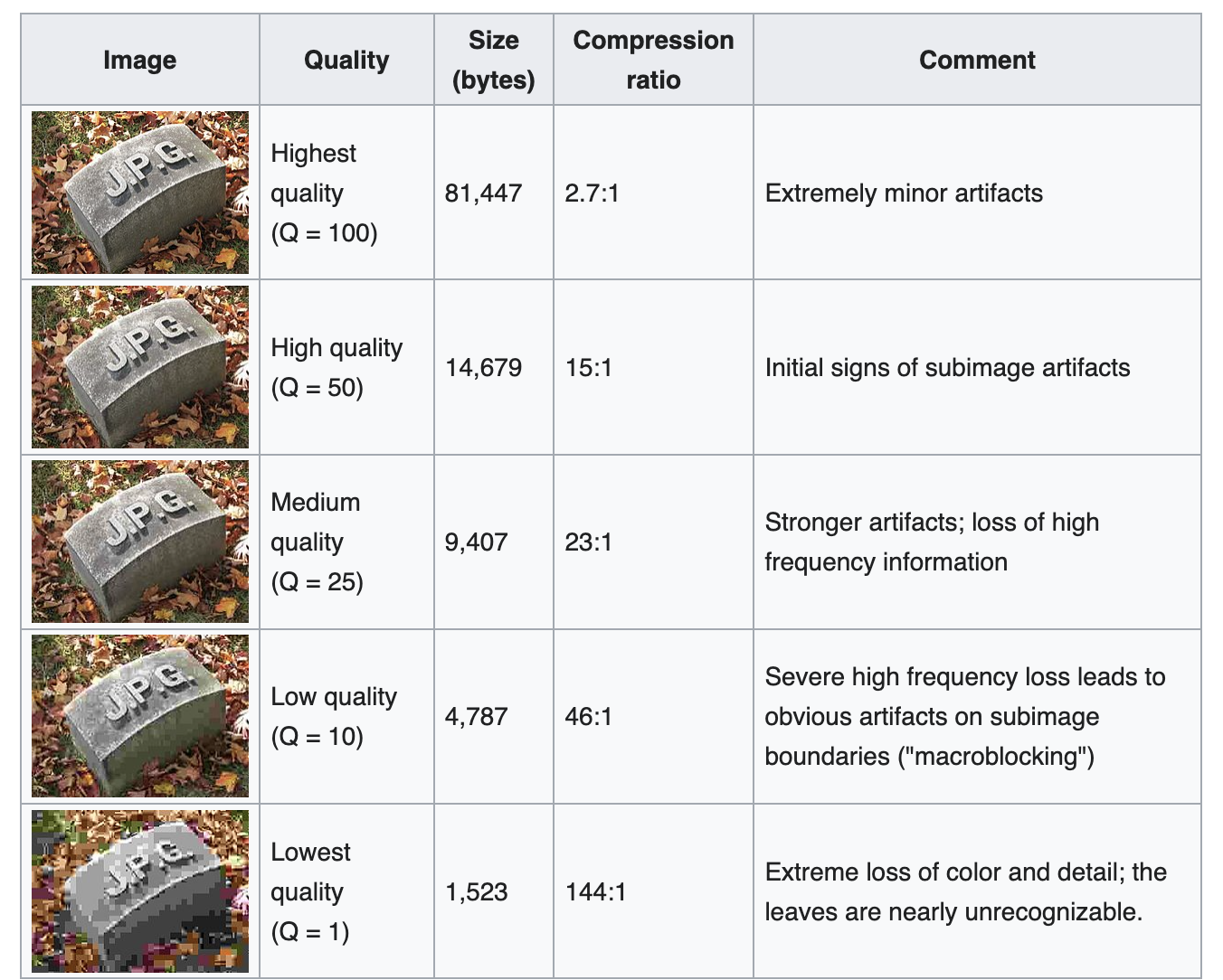
  • Lossy compression is often used for photos, audio, and video in situations in which absolute accuracy isn’t essential. Most of the time, we don’t notice if a picture, song, or movie isn’t perfectly reproduced. The loss in fidelity becomes more perceptible only as files are squeezed very tightly. In those cases, we notice what are known as compression artifacts: the fuzziness of the smallest jpeg and mpeg images, or the tinny sound of low-bit-rate MP3s.
  • JPEG gets around it by only choosing ‘visually important’ information to keep and either keeping around lower quality version of it or dropping it altogether
  • Two main principles:
    1. Changes in brightness are more important than changes in colour: the human retina contains about 120 million brightness-sensitive rod cells, but only about 6 million colour-sensitive cone cells.
    2. Low-frequency changes are more important than high-frequency changes: we notice the boundaries of objects much more easily than the fine detail and patterning on it.

Encoding

Colour Transformation

(yes with a u)

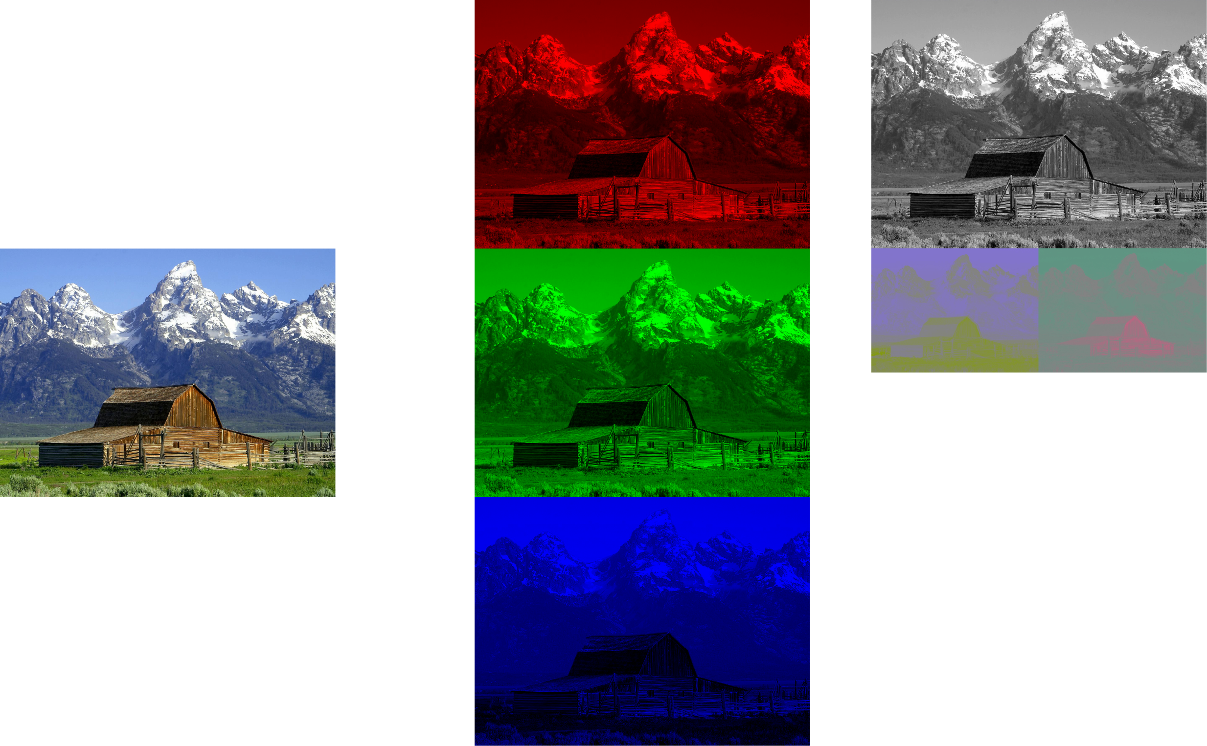
• Normally, image information in computers are stored as pixels ([W, H, 3])
  • 3 Channel — R, G, B
  • However, the image’s brightness information is spread evenly through the R, G, and B channels.
    • Each channel value is from 0 to 255 for brightness of that colour.
• One optimization we can do is decreasing the bandwidth or resolution allocated to “color” compared to “black and white”, since humans are more sensitive to the black-and-white information. This is called chroma subsampling.
  • Old televisions used to do this because RGB was way too redundant so they wanted something that compressed better.
  • Originally for standard-definition television use in the ITU-R BT.601 standard for use with digital component video
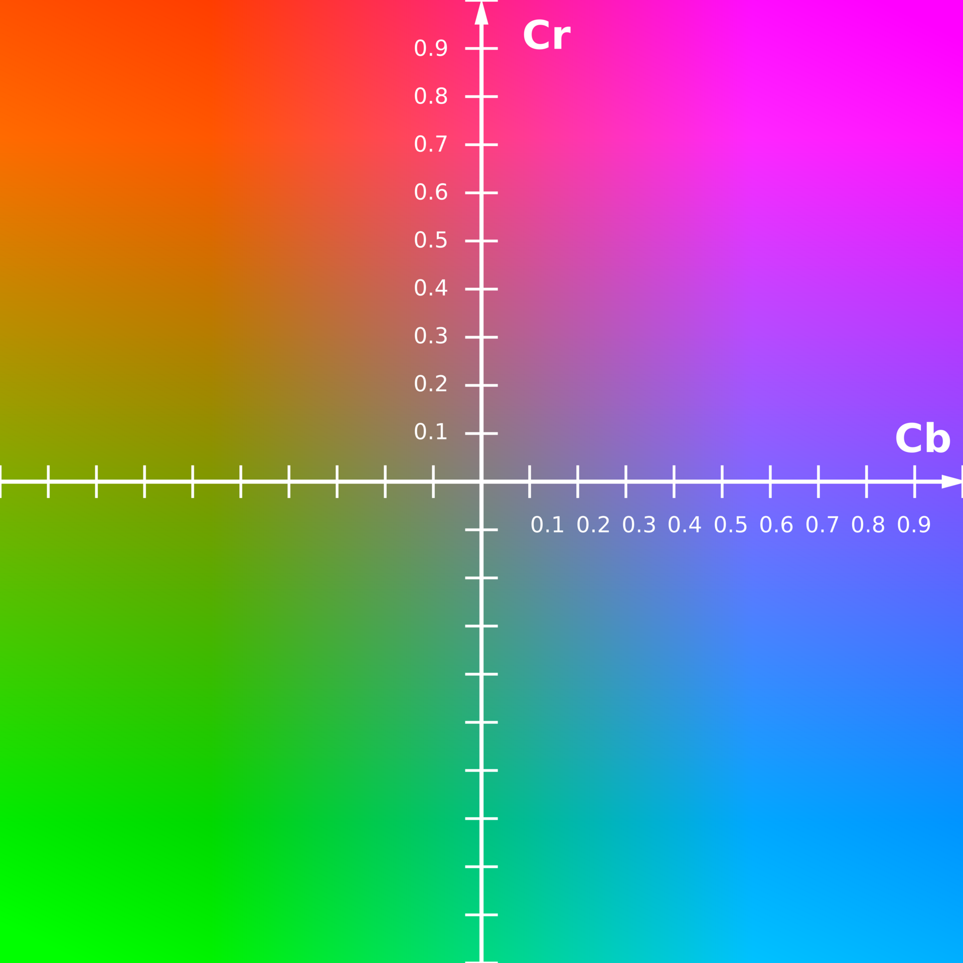
• JPEG converts from RGB colour space to YCbCr
  • Y is the luma (brightness) component and Cb and Cr are the blue-difference and red-difference chroma (colour) components
    • Y normally has a range of 0 to 1
    • Cb and Cr normally have a range of -0.5 (negative amount of the colour) to 0.5 (positive amount of the colour

For this example, after keeping only a quarter of the colour information, we already reach a 2x compression ratio. Notice that we started with 3 full channels and now we have 1 full channel and 2 × ¼ channels!

Spatial to Frequency Domain

Finally, a tangible use-case for a Fourier transform! Specifically, the Discrete Fourier Transform.

• Go from a signal to its component parts
• We are trying to decompose something complex into a sum of simple things

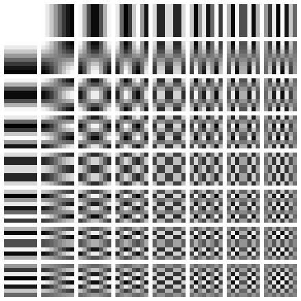
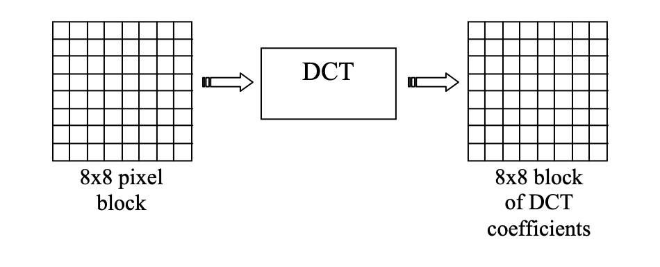
JPEG does this but in 2D for each of the YCbCr channels. We chunk up an image into 8x8 ‘blocks’ and then decompose it into some basic patterns that are made up of cosines with various periods.

Note

If the data for a channel does not represent an integer number of blocks then the encoder must fill the remaining area of the incomplete blocks with some form of dummy data. Most of these techniques cause artifacts (see: Boundary Effects) but generally repeating the value at the edge works well enough.

Here are the following 64 ‘principle’ components that it uses:

Note

The top-left block is the ‘basic hue’ and is often called the DC component. The other 63 blocks are called AC components.

The top left being a completely constant block and the bottom right being the most ‘detailed’ texture.

We end up with a table of DCT coefficients for each of the channels Y, Cb, and Cr.

Quantization

If you have ever saved a JPEG image and chosen a quality value, this is where that choice comes into play.

Here, we can toss away some of the information from the previous step because we know we have the principle where low-frequency changes are more important than high-frequency changes.

JPEG has separate 8x8 quantization tables of how much to divide the coefficient tables by. The lower quality of JPEG we choose, the larger the value in the quantization tables. The values range from 1 (preserve all the detail, highest quality) to almost 800 (pretty much set the coefficient to 0, ignore it entirely, lowest quality). After dividing the frequency values by these coefficients we quantize it to the nearest whole number. This effectively ‘squashes’ the range of the frequency values.

Note that these values are not uniform across the 8x8 quantization table. Generally, the coefficients are smaller in the top-left and get larger as you go diagonally to the bottom-right. This has the effect of squashing the high-frequency coefficients to 0.

Note

This is where most of the information loss happens. It also is how ‘deep-frying images’ happens:

Lossless compression

Even after the quantization step, we still have the same amount of data: one number for each pixel from each of the three channels. However, what it does enable is for us to apply this next step much more efficiently.

You can see why here:

   n = 0, 1, 2, 3, 4, 5, 6, 7, 8, 9, 10, 11, 12, 13, 14, 15, 16, …
 n/2 = 0, 1, 1, 2, 2, 3, 3, 4, 5, 5,  5,  6,  6,  7,  7,  8,  8, …
n/16 = 0, 0, 0, 0, 0, 0, 0, 0, 1, 1,  1,  1,  1,  1,  1,  1,  1, …

It’s much easier to write an algorithm that can compress the bottom sequence than the top one.

JPEG uses 3 fun techniques here:

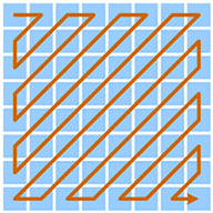
Unwrapping blocks in zig-zag order

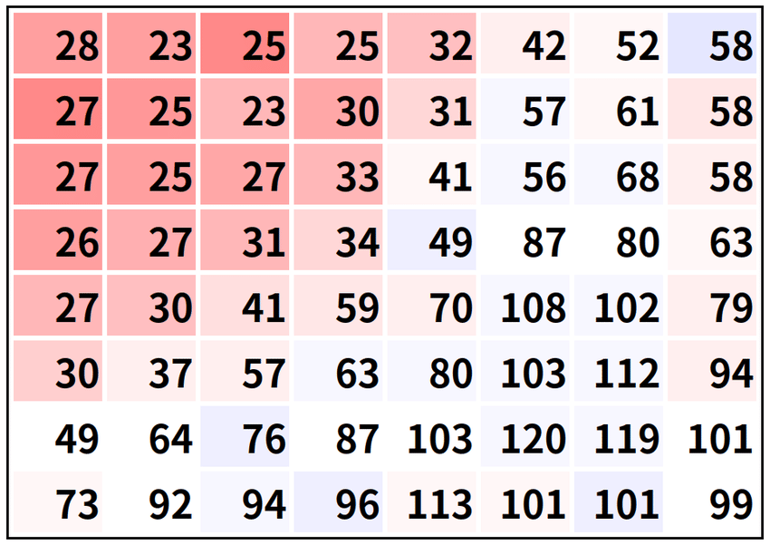
In each block, we know that we have a rough diagonal trend of values that start high in the top-left and get progressively closer to zero as we move to the bottom-right.

Some genius was like ‘holy cow’, if we read the squares in a zig-zag pattern, we can minimize the delta between each value that we read and get more efficient compression!

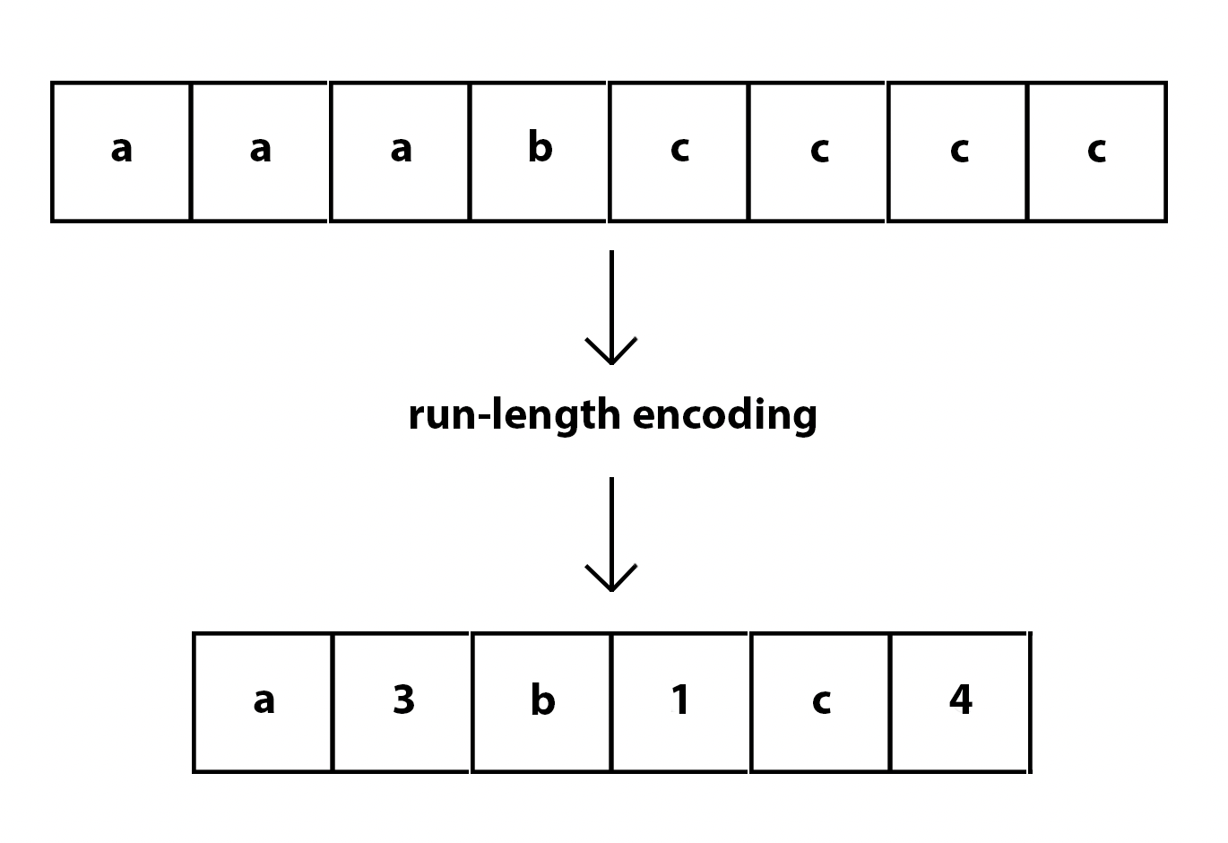
Run-length encoding and Huffman coding

These are pretty standard compression techniques so I won’t dive too deep into these here.

Run-length encoding allows us to transform repeated sequences into how many times the thing was repeated

Huffman coding picks up where run-length encoding ends off.

It’s a form of variable-length encoding that takes advantage of information theory to encode common components of the input based off of the frequency at which they occur.

More frequent patterns get shorter codes (similar to how Morse code works). Zipf’s law helps to explain why this is so effective:

In a sorted list, the value of the $n$th entry is inversely proportional to $n$.

It turns out that in the vast majority of cases, in a sequence in integers, the most frequent integer occurs approximately twice as often as the second most frequent integer, three times as often as the third most frequent word, and so on.

So, by taking only 2 or 3 bits to encode the ‘most common’ numbers (even compared to using 8 bits to represent an unsigned integer which can only represent numbers from 0 to 255), we can compress quite a bit!

Decoding

All the above, but in reverse!!

Because we threw out a lot of information in the chroma subsampling and quantization steps, we cannot perfectly reconstruct the original image (hence, lossy compression!).