Object Classification

See also: object detection

Data to Model

Random Sample Consensus (RANSAC)

1. randomly choose minimal subset of data points necessary to fit model
2. points within some distance threshold of model are a consensus set, the size of the consensus set is the model’s support
3. repeat for N samples, model with biggest support is most robust fit

Choosing number of samples $k$

1. let $\omega$ be the fraction of inliers
2. let $n$ be the number of points needed to define hypothesis (e.g. $n=2$ for a line)
3. suppose $k$ samples of $n$ points are chosen. then
   1. the probability that all $n$ in a sample are correct is ${\omega }^n$
4. the probability that all $k$ samples fail is $(1-{\omega }^n{)}^k$, thus we choose a $k$ large enough to keep this below a targe failure rate

Advantages

• general method
• easy to implement and calculate failure rate Disadvantages
• only handles a moderate percentage of outliers without cost blowing up
• many real problems have high rate of outliers (e.g. noise)

Hough Transform

• For each token, vote for all models to which the token could belong
• Return model with most votes

e.g. for each point, vote for all lines that could pass through it; true lines will pass through many points and thus receive many votes

Turning image space into parameter space. Rearranging $y=mx+b$ into $y-mx=b$ where $b$ and $m$ are the variables instead of $y$ and $x$.

We can alternative transform it using Book’s Convention: $x\sin (\theta )+y\cos (\theta )+r=0$. Then, $x\sin (\theta )+y\cos (\theta )=\rho$

Advantages

• Can handle high percentage of outliers: each point votes separately
• Can detect multiple instances of a model in a single pass Disadvantages:
• Complexity of search time increases exponentially with the number of model parameters
• Can be tricky to pick a good bin size

Classification

Classifier is a procedure that accepts as input a set of features and outputs a prediction for the class label.

Standard Bag-of-Words pipeline

1. Dictionary Learning: learn visual words using clustering
2. Encode: build Bags-of-words vectors for each image
3. Classify: train and test data using BOW (KNN, naive Bayes, SVM)

Bayes Rule

See: Bayes’ Theorem

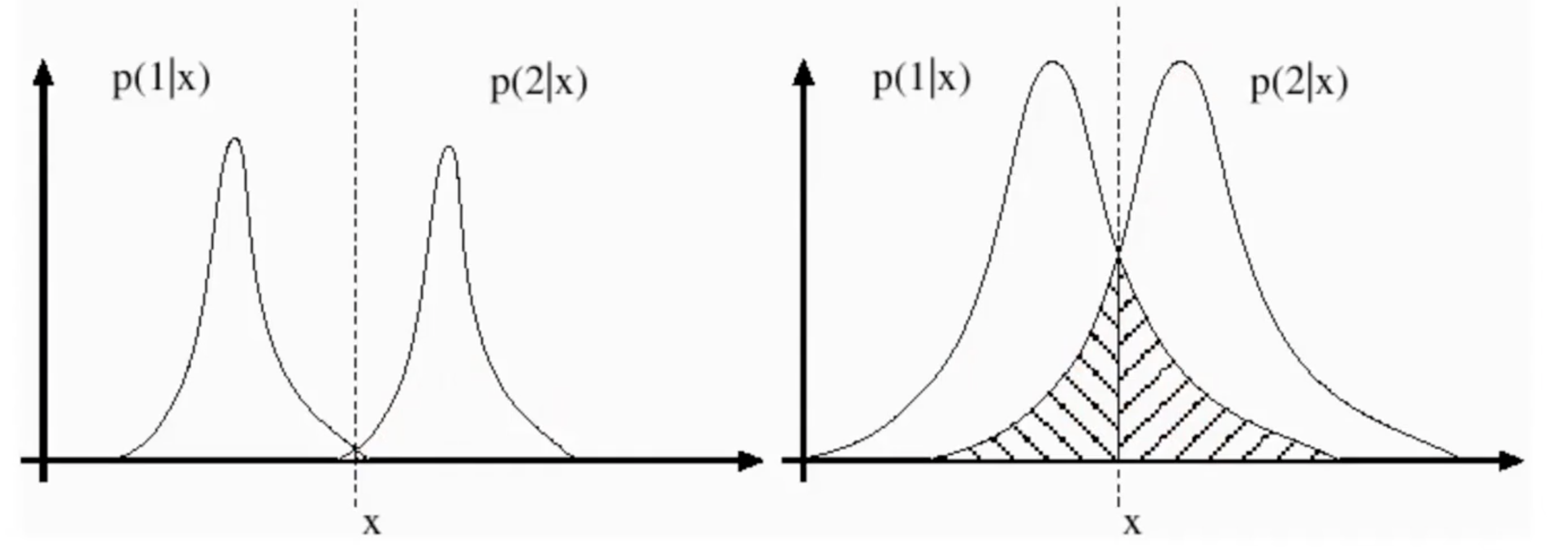
Decision boundary, the location where one class becomes more probable than the other (e.g the point where the probability classes are equal).

The Bayes’ risk is the shaded region where one class’s probability is still non-zero beyond its decision boundary.

See also: probability

ROC Curve

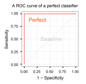
Trade-off between true positive rate and false positive rate. A random classifier will always have 1:1 true positive and false positive rate

Parametric vs Non-parametric

• Parametric classifiers rely on a model
  • fast, compact
  • flexibility and accuracy depend on model assumptions
• Non-parametric classifiers are data driven (rely on comparing to training examples directly)
  • slow
  • highly flexible decision boundaries

Spatial Pyramid

Have multiple scales of the input image to compute histograms across. Train a classifier for each scale along with a combined weight to combine each classifier.

VLAD (Vector of Locally Aggregated Descriptors)

Instead of incrementing the histogram bin by a single count, we increment it by the residual vector $x-c(x)$ (diff between cluster center and feature vector)

Dimensionality is $Kd$ where $K$ is number of codewords and $d$ is the dimensionality of the local descriptor (128 for SIFT)

Decision Tree

See notes on decision trees

Classifier Boosting

• Train an ensemble of classifiers sequentially
• Bias subsequent classifiers to correctly predict training examples that previous classifiers got wrong

CNNs

See notes on CNNs