 How do we tell that this is a “valid” intent?
A (not so) brief exploration of how we tackle classifying intents in reflect. Part 1 will touch on defining the problem we’re trying to solve, the data we have, and how we pre-processed it. Part 2 will focus on the architecture of the model we built, how well it does, and thoughts on improving it for the future.
The problem
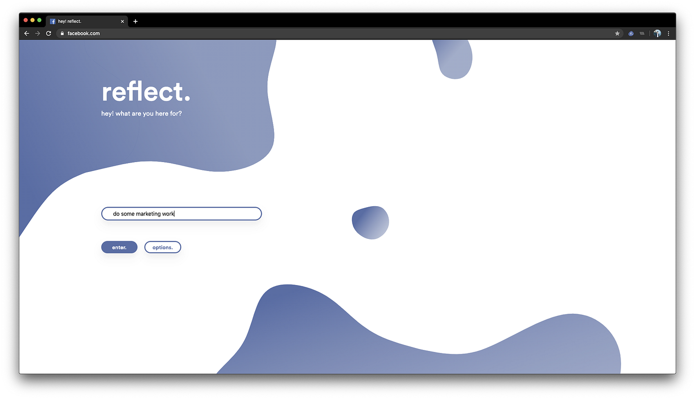
Classifying intents is at the core of reflect. When a user inputs an intent, its reflect’s job to figure out whether that intent should let them into the website.
How do we make sure “do some marketing work for reflect” is classified as productive but “watch cute dog videos” isn’t?
Why it’s so difficult
A lot of it comes down to the fact that natural language processing (NLP) is a very difficult task. What does the sentence “learn about physics” mean, and how is it semantically different from “asdflkj I can’t do work”?
We can’t just parse for keywords and just allow a user in if we see the word “work” because that word can mean different things in different contexts. For example, “I’m not doing any work right now” would have otherwise been classified as valid. Thus, we can employ the help of a machine learning algorithm to help us capture this deeper meaning.
Specifically, the form of machine learning we will be using is called supervised learning, in which we give an algorithm a bunch of labelled data, tell it what it’s doing wrong, and let it ‘learn.’ Through doing this, hopefully the algorithm will be able to generalize and make predictions on unseen data too.
The data
Of course, if we want to perform supervised learning, we’re going to need a lot of data. Where are we going to get all of it? Luckily, we were able to get it through 3 different sources.
Survey data (444 entries)
Our team sent out an interest survey in early January in which we asked 3 questions:
- How would you answer if you were trying to visit a distracting site while trying to focus? (eg. youtube, facebook, etc)
- How would you answer if you were trying to visit a distracting site to take a quick break from your work? (eg. youtube, facebook, etc)
- How would you answer if you were trying to visit a distracting site like Facebook but to do work? (e.g. make a marketing post)
We used these answers to form the basis of our very first dataset. We ended up getting a surprising amount of entries, ending with 148 responses to 3 questions and totalling 444 different observations. Here’s what some of that data looks like after tidying it up:
We classified any answer to Q1 as invalid and Q2 + Q3 as valid
| intent | valid |
|---|---|
| I am watching a 5 minute video to take my mind off not being productive :/ | no |
| I’m just bored | no |
| I’m bored/tired and trying to relax | no |
| … | … |
| work is pretty boring, i need to take a quick break I just can’t focus atm | yes |
| I finished all my work for today so I’m going to take a break now! | yes |
| getting some advertising done for my club | yes |
| I need to make a post on Twitter for my job announcing the latest update to our site | yes |
| I’m trying to network | yes |
| … | … |
Closed Beta (790 entries)
After we made a basic dataset, we were able to make our first (admittedly not great) model. But in doing so, this let us create an MVP to which we could use to actually test with. We then deployed this model for use to our closed beta testers and collected their responses (with consent of course!) along with the website it was input on. This was then converted into a .csv file. A few examples are show below:
| intent | url |
|---|---|
| to do some marketing | facebook.com/ |
| i cannot focus on my work | instagram.com/ |
| fuel my crippling social media addiction | facebook.com/ |
| … | … |
These were then hand-labelled by our reflect team in a similar format as the survey data we collected earlier.
| intent | valid |
|---|---|
| to do some marketing | yes |
| i cannot focus on my work | no |
| fuel my crippling social media addiction | no |
| … | … |
Closed Beta Corrections (37 entries)
Finally, we created a Google Forms through which we directly asked beta testers if a decision made by reflect’s intent classifier was faulty. Specifically, we asked what they input, and what they expected. Here are a few examples:
| input | valid |
|---|---|
| reply to a friend about a lab | yes |
| listening to a youtube music playlist | yes |
| goof off as much as possible | yes |
| … | … |
This entire section of the dataset was only 37 observations, but it drastically helped us reduce false positives and false negatives by focusing specifically on misclassifications.
After aggregating and combing all our data into one common format, we ended up with a grand total of 1271 observations. They looked something like this:
| input | expected |
|---|---|
| fail school by watching youtube | no |
| sdlkjasd | no |
| making a quick product post (should take <10 min) | yes |
| … | … |
So?
Now that we have the data, can we just throw it into a machine learning model? Unfortunately, the answer is no, not quite yet.
Data augmentation
Our dataset is still pretty small, even after aggregating all of our data. It most definitely doesn’t cover all of our bases for all the possible things that future users could possibly input. So, how can we “upsample” our data to get more of it? Well, it turns out that the field of Natural Language Processing has quite a few tricks to augment our data.
Sentence Variation
Essentially what sentence variation is, is just replacing a few words of given sentences with their synonyms. If we have a sentence like “I’m trying to make a marketing post,” we can swap out singular words with their synonyms and tell our network that it means the same thing.
In this example, we could get something like “I’m attempting to fabricate a marketing post”. Adding these additional sentence variations will allow our machine learning model to learn semantic relationships between similar words (e.g. fabricate and make have similar meaning)
Sentence Negation
Additionally, if we add a ‘not’ in the sentence, it should flip the meaning of the sentence. An example would be “learning about physics” is valid, whereas “not learning about physics” is not. However, if the sentence already contains ‘not’ (e.g. “I’m not being productive”), adding another ‘not’ would make the sentence too complex and obfuscated, so we just label it as invalid. In essence, we just add ‘not’ to a bunch of sentences and label them as invalid. This helps us to combat intents which use negations in a sort of round-a-bout way to confuse the algorithm.
Shuffled Sentences
If we take an existing, valid sentence and completely shuffle the words, the resulting sentence should be invalid. An example would be “to watch a crash course video*” should be valid whereas “video course a watch crash to*” should be invalid. Basically, we’re just shuffling existing sentences and also labelling them as invalid. This helps us to combat intents which grammatically make no sense, but are otherwise valid.
Garbage Sentences
We can also take completely random words from the English language and put them together. The resulting sentences should all be invalid. For example, “*untinkered phalangitis shaly quinovic dish spadiciflorous unshaved” *clearly makes no sense. However, the addition of these gibberish sentences allows our model to be more robust against foreign words and out-of-vocabulary terms.
Vocabulary-mix Sentences
Last but definitely not least, we can take the most common words in our dataset and mash them together. This should yield us a bunch of sentences which contain “key words” but should be marked as invalid because the context in which they are used makes no sense. For example, “video look watching” and “get research facebook take need want need message watch” are both clearly gibberish sentences, but they have a lot of keywords that one would think would let you in (e.g. video, research, watching, etc.). This lets us be more robust against those who try to get around the algorithm using keywords.
Data preprocessing
What about now? Can we throw it into the neural network yet? Well, no. We may have increased the amount of data we have to work with, but we also need to convert it to a form that is easy to understand for both the computer and for our algorithm. We do that with a series of functions that we apply on our data.
Strip punctuation
As the name suggests, we remove all punctuation from the input phrase. We found that including the punctuation hurt our performance, most likely due to the fact that they offer very little in terms of semantic meaning and obfuscate the real meaning of the sentence.
stripPunctuation("I don't know if I'm being productive! :(")
> "I dont know if Im being productive"
Make everything lowercase
Additionally, we found that in this particular setting, capital letters also didn’t matter that much. Because of the nature we collect our data (just a simple textbox), users tend to not bother with capitalization. As such, we remove it to make it consistent across our data.
lower("I dont know if Im being productive")
> "i dont know if im being productive"
Expand contractions
The English language does this weird thing where we can just smush two words together (e.g. “I am” to “I’m”). Unfortunately for us, these produce extra complexity in our model that we could reduce by making them all consistent. In our case, we chose to expand all of these contractions.
expandContractions("i dont know if im being productive")
> "i do not know if i am being productive"
Remove stop words
The English language also has a bunch of these things called stop words — words that do not contribute anything major to the sentence in terms of semantic understanding (usually in the context of natural language tasks such as this). A few examples of them are ‘I’, ‘me’, ‘my’, ‘by’, and ‘on’. By removing them, we once again remove unneeded complexity from the model.
rmStopwords("i do not know if i am being productive")
> "not know productive"
Tokenization
However, these words are not super friendly for machine learning algorithms who would much rather deal with integers and floating point numbers than words and sentences. How do we fix this?
Well, one thing we can do is turn words in indices by how often they appear, capped at the most common 1000 words — in essence, creating a vocabulary list mapping common words to numbers. For example, if “the” is the most common word, we convert it to 1. If “work” is the 8th most common word, we convert it to 8. For anything that isn’t in the top 1000, we give it the value of 0.
tokenize("not know productive")
> [12, 35, 7]
Fixed sequence length
Finally, we need to ensure that all the inputs are the same length of simplicity sake. If we were to handle dynamic length inputs, it would introduce a whole other level of complexity that we’re really not ready to deal with. As such, we can make sure all the inputs are the same length by adding a bunch of zeros to those who are too short (zero padding) or by slicing those who are too long.
pad([12, 35, 7], 10)
> [0, 0, 0, 0, 0, 0, 0, 12, 35, 7]
Finally
After all of these functions have been applied, we have successfully converted a complex sentence into a series of ‘tokens’ that is easy to understand for the machine learning algorithm.
preprocess("I don’t know if I’m being productive! :(")
> [0, 0, 0, 0, 0, 0, 0, 12, 35, 7]
What’s next?
Now that we have something ready to feed into our neural network, let’s dive into how the actual model itself works! How do we tell that this is a “valid” intent?
The model
The type of neural network that we’ll be using is called Long Short-Term Memory (LSTM).
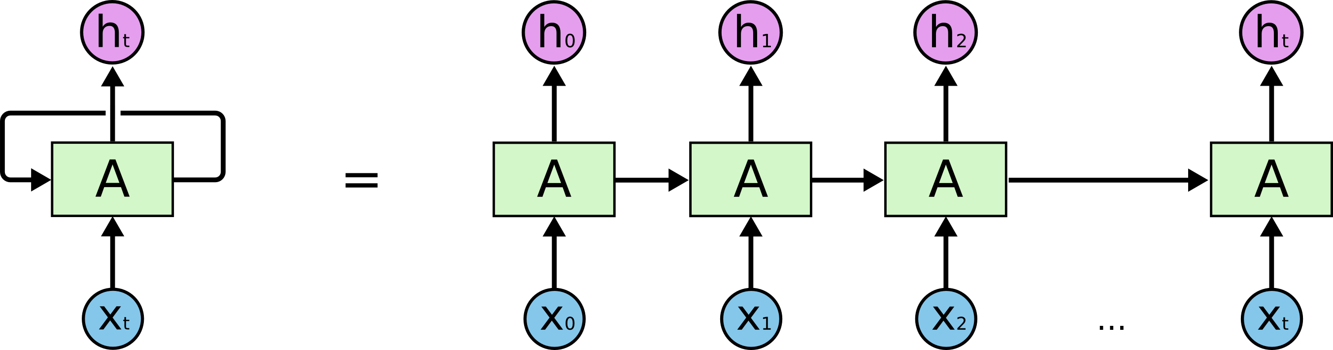
What’s so special about these networks is that they are really good at modelling time-series data, making it an ideal candidate for tasks like forecasting or natural language processing.
# Function to create a RNN model with given parameters
# max_seq_len: maximum token sequence length
# vocab_size:  size of tokenizer vocabulary
def RNN(max_seq_len, vocab_size):
    inputs = Input(name='inputs', shape=[max_seq_len])
    layer = Embedding(vocab_size, 64, input_length=max_seq_len)(inputs)
    layer = LSTM(64, return_sequences = True)(layer)
    layer = Dropout(0.5)(layer)
    layer = LSTM(64)(layer)
    layer = Dense(256, name='FC1')(layer)
    layer = Dropout(0.5)(layer)
    layer = Dense(1, name='out_layer')(layer)
    layer = Activation('sigmoid')(layer)
    model = Model(inputs=inputs, outputs=layer)
    return model
Here’s how we define it in our Keras code, don’t worry if you don’t understand it just yet! We’ll explain it in the next few paragraphs.
inputs = Input(name='inputs', shape=[max_seq_len])Right off the bat, you’ll notice that the first layer is the Input layer. Basically, this tells Keras to instantiate a new tensor (a multi-dimensional vector) with a given shape. In this case, we’re creating a one-dimensional tensor that is max_seq_len units long. When we trained our model, this was set to 75.
layer = Embedding(vocab_size, 64, input_length=max_seq_len)(inputs)Next up, we have the Embedding layer. We could get into a really technical discussion about what this really does, but you can think of it as a layer that helps the neural network to learn semantic relationships between inputs.
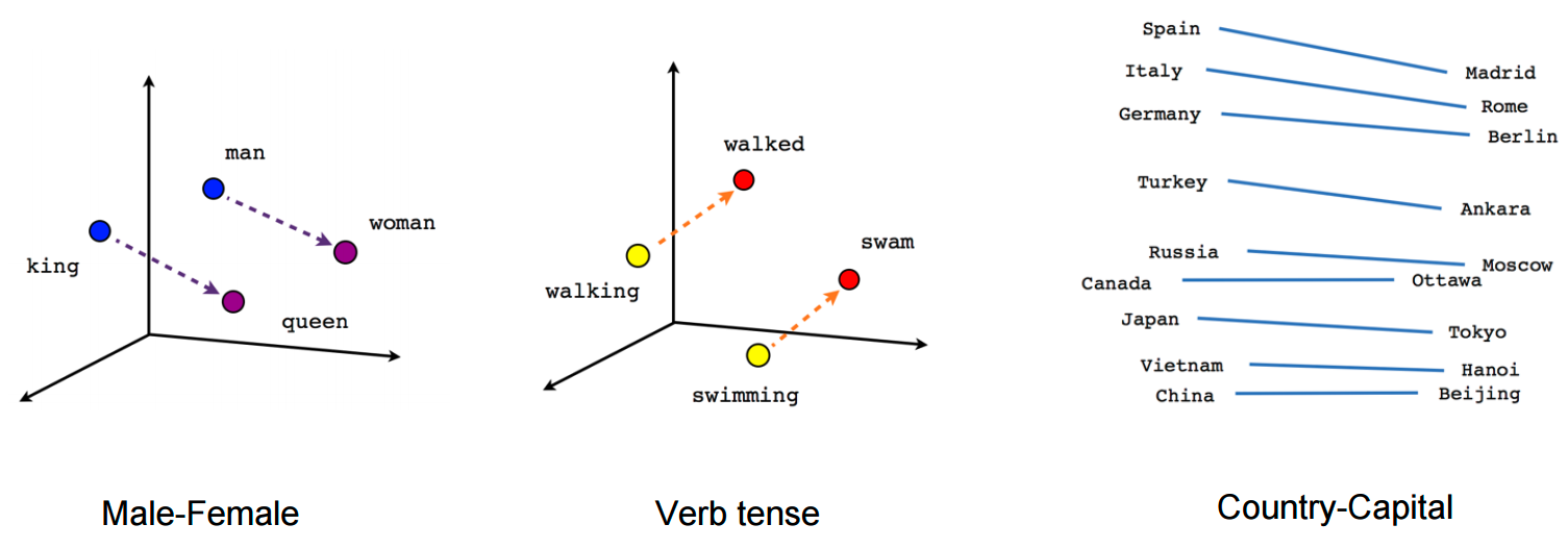
Essentially, it embeds tokens in a higher dimension vector space, where distance between tokens represents its similarity.
layer = LSTM(64, return_sequences = True)(layer)Now, we get into the meat of the neural network: the LSTM layer. As stated before, these LSTM networks are really good at modelling time series data like language. In this case, our LSTM network has 64 hidden units per cell, and that we’d like to pass these hidden states to the next layer. If you’d like to learn more about the inner workings of the LSTM model, theres a really good resource here!
layer = Dropout(0.5)(layer)Next, you’ll notice there are a few Dropout layers. These layers help to prevent overfitting by randomly killing off connections between the two layers (a sort of regularization). This makes sure neurons aren’t just “memorizing” the input data. This is especially important because our dataset is relatively small (~2000 observations even after augmentation), so making sure that our machine learning model can generalize outside of this limited dataset is really important.
layer = LSTM(64)(layer)We have yet another LSTM layer! By having these two chained right after each other, the first layer can pass all the values of all of its hidden states to the second layer, effectively allowing a sort of ‘deeper’ neural network.
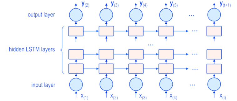
This deep LSTM allows our network to learn more abstract concepts, making them well suited for natural language tasks.
layer = Dense(256, name='FC1')(layer)Next, we have something called a Fully Connected layer, or a Dense layer. In a dense layer, each of the input neurons is connected to every output neuron. This kind of ‘glue’ layer helps the network to pick out and discriminate feature output by our previous LSTM layer.
layer = Dense(1, name='out_layer')(layer)
layer = Activation('sigmoid')(layer)
Similarly, we have one final Dense layer that ‘compresses’ all of the hidden units down to one neuron. However, we want the output value of this neuron to be how confident from a scale of 0 to 1 it is that the intent is valid. We do this by applying something called an activation function.
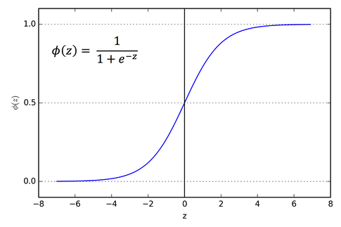
In this case, the particular function we chose is the sigmoid activation function, which looks something like the above.
Model Overview
Phew, finally got through everything! After putting it all together, we end up with a network that looks something like this:
# 75 max_seq_len
# 1000 tokenizer_vocab_size
model = net.RNN(75, 1000)
model.summary()

# _________________________________________________________________
# Layer (type)                 Output Shape              Param #
# =================================================================
# inputs (InputLayer)          (None, 75)                0
# _________________________________________________________________
# embedding_1 (Embedding)      (None, 75, 64)            64000
# _________________________________________________________________
# lstm_1 (LSTM)                (None, 75, 64)            33024
# _________________________________________________________________
# dropout_1 (Dropout)          (None, 75, 64)            0
# _________________________________________________________________
# lstm_2 (LSTM)                (None, 64)                33024
# _________________________________________________________________
# FC1 (Dense)                  (None, 256)               16640
# _________________________________________________________________
# dropout_2 (Dropout)          (None, 256)               0
# _________________________________________________________________
# out_layer (Dense)            (None, 1)                 257
# _________________________________________________________________
# activation_1 (Activation)    (None, 1)                 0
# =================================================================
# Total params: 146,945
# Trainable params: 146,945
# Non-trainable params: 0
# _________________________________________________________________
Theres a grand total of 150,000 different trainable knobs and parameters in our neural network!
Training pipeline
So, how does the data we got earlier play a role in helping our machine learning model learn and improve?
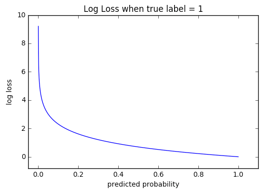
The first component is the loss function. This component tells the neural network how ‘correct’ its prediction was. In this model, we will use something called binary cross entropy, which is basically a fancy word for log-based error. If the true label is 1, we can then show what the log-loss would be for some given prediction probability.
Next, we need to pick an optimizer. This component tells the neural network how to change its parameters to improve or ‘optimize’ itself. In this model, we chose to use an optimizer called RMSProp with a learning rate of 1e-3 . We aren’t going to cover all the technical details of this optimizer in this blog post, but just know that it is a very fast and effective optimizer.
 RMSProp(black) vs a bunch of other optimizers. credit: Vitaly Bushaev
One important hyperparameter we choose is the train-test split. In data science and machine learning, we typically withhold part of our data and set it aside as a test set. The rest of the data will be considered the training set. When training the model, we never feed it the test set. As a result, we can use the test set as a metric to see how well it would perform on real-world, unseen data. In our training, we used a train-test split of 20%.
Another important hyperparameter that we can choose is the mini-batch size. The mini-batch size determines how many training examples we feed the machine learning model before updating its parameters. A smaller mini-batch means that we get more frequent updates to the parameters, but it also runs the risk of having outliers that may cause a bad gradient update. A large mini-batch means that we get a more accurate gradient update but it also takes longer. A similar concept is sample size in statistics. We could pick a larger sample to get a better estimate of the overall population, but it is often more expensive to do so. A smaller sample might contain outliers and thus be less robust of an estimate of the overall population, but it very easy to do. So, there’s this tradeoff between accuracy and speed. We found that a good balance between these was a mini-batch size of 128.
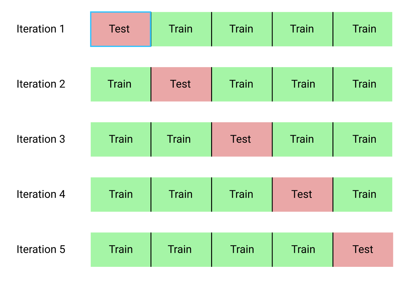
We then trained our neural network over 10 epochs. A single epoch is one iteration over the entire dataset. If we train it for too many epochs, you run the risk of overfitting (memorizing the training data), but we don’t train it enough, we run the risk of not discovering a better model. One thing we can do it minimize this problem is through the use of cross-validation, which is a technique that lets us ‘test’ on portions of the training set. Essentially, at each iteration during training, we withhold a portion of the training set and use it as a sort of ‘validation’.
 credit: Raheel Shaikh
By seeing when this validation accuracy goes down, we can get a pretty good idea of when our model begins to overfit on our data, and stop the training before this happens. In training our model, we will use 5-fold cross-validation.
After all of this, we end with a training accuracy of 93.60% and test accuracy of 85.95%. Not bad at all!
Serving the model
Great! So now we have a trained model. Can we put that in the Chrome extension now? Not quite yet…
Our model was written and trained with Keras (a Python Deep Learning library). Our Chrome extension is written in TypeScript. How do we get these two to work together?
Luckily for us, Tensorflow.js exists! This library allows us to run Tensorflow models from within JavaScript. Tensorflow has released a script that lets us to convert a Keras model into something that Tensorflow.js understands, so we can run that to convert our models.
However, we can’t just directly plug-and-play. You may remember that we did all of that data preprocessing before we trained our model. Tensorflow.js doesn’t have any of this built in, so we made our own implementation of it. You can check it out here.
We’ll leave all the technical code out (if you’re interested, feel free to peek around the source code!), but we’ve abstracted it enough that classifying an intent is a breeze.
// declared somewhere earlier
const model: nn.IntentClassifier = new nn.IntentClassifier("acc85.95") // name of converted model

// send to nlp model for prediction
const valid: boolean = await model.predict(intent)
if (valid) {
  // let through
} else {
  // block page
}
Future improvement
Possible models
We have thought about using something more established and complex like BERT and retraining it on our dataset, however then comes the problem of runtime and memory usage.
BERT is a huge model. If you thought 150 thousand parameters was a lot, wait till you see BERT’s 110 million parameters. This bad boy takes a few hundred times longer and many times more memory than our current model. While yes BERT may perform really well, we just don’t think it has a place inside of a Chrome extension.
Our model is decently robust as it is, especially considering the entire model is <2MB and takes less than 200ms to run in browser. For now, we will stick with lightweight models, but we may switch if we find a better match in the future :)
Misclassifications
Of course, this algorithm isn’t perfect. It does have a lot of flaws and weaknesses that we find every day, and we’re working to fix those! If there are any misclassifications that you find in the algorithm, we love to hear about it on our feedback form: https://forms.gle/ctypb6FmDT9RQqjv6.
Closing
This NLP model is at the core of reflect. It is this model’s goal to predict whether user intents are valid or not. As a result, we need to make sure this algorithm is accurate, fast, and lightweight. Hopefully, through this blog post, you’ve learned a little about how we went about building a model to fulfill those requirements.
Learn more about us on our website! ✨ http://getreflect.app/
If you have any further questions about reflect or this NLP model, feel free to shoot us an email at [email protected]