Transformer Models

See also: LLMs, NLP

At a high-level, we can think of a transformer model as taking an input sequence of tokens of length $n$ and predicting the next token at index $n+1$. They generally excel at sequence-to-sequence modeling tasks.

Most implementations of transformers are autoregressive, meaning that it predicts future values (index $n+1$ to $\infty$) from past values (index $0$ to $n$).

Inference

Mainly derived from Brendan Bycroft’s amazing LLM visualization

Embedding

The smallest unit of understanding for a transformer is a token. This is usually a common sequence of characters like ‘at’ or ‘qu’.

The collection of all the tokens the model understands is its vocabulary. The vocabulary maps the token to its index:

• Token A: index 0
• Token B: index 1
• Token C: index 2

This lookup table is usually trained or determined independently of the LMM itself. Most people use statistical methods based on the data to figure out a good lookup table. One common example of this is BPE.

The first step of a transformer is turning the input text into the appropriate index in the vocabulary table.

Then, we use the token index to select the associated column in the token embedding matrix (e.g. the 3rd token index corresponds to the 3rd column of the token embedding matrix). The values of the token embedding matrix are vectors which we call the token embeddings. The token embedding matrix is $[C_{\text{embed}},n_{\text{vocab}}]$ where $C_{\text{embed}}$ is the dimensionality of this embedding.

Then, based on the index of the token in the input, we use it to select an appropriate column of the position embedding matrix. The dimensionality of this is the same as $C_{\text{embed}}$. We need position embeddings because, unlike RNNs and LSTMs which operate sequentially, Transformers operate over the whole input sequence at once so it loses information related to token order.

Why can't we just use a column vector of what index the token is?

A few good criteria for a positional embedding function:

• It should output a unique encoding for each time-step (word’s position in a sentence)
• Distance between any two time-steps should be consistent across sentences with different lengths.
• Our model should generalize to longer sentences without any efforts. Its values should be bounded.
• It must be deterministic.

We try to regularize our weights to ensure they stay close to zero (but not zero exactly!). This would disproportionately distort the embeddings of later tokens! Even if we embed it as a fraction of the total sequence length (so that the position embedding for the first token is a column-vector of $0$ and the $1$ for the last token), that wouldn’t work either as for different lengths of inputs, we would get different position embeddings for the same token position.

The people who wrote the original Transformer paper “Attention Is All You Need” came up with a very smart way of representing position by using:

• $P{E}_{(pos,2i)}=\sin (pos/10000^{2i/C_{\text{embed}}})$ for even dimensions and
• $P{E}_{(pos,2i+1)}=\cos (pos/10000^{2i/C_{\text{embed}}})$ for odd dimensions

The key part for avoiding collisions was the fact that the wavelength changes depending on $i$, the dimension. Even if the positional encoding of the first dimension of position $x$ and position $y$ are the same (due to periodicity in sinusoidal functions), it is very unlikely that given a reasonably high $C_{\text{embed}}$, we get the same positional embedding for different $i$.

The intuition for this comes from how we represent numbers in binary.

0. 0000
1. 0001
2. 0010
3. 0011
4. 0100
5. 0101
6. 0110
7. 0111
8. 1000
9. 1001
10. 1010
11. 1011
12. 1100
13. 1101
14. 1110
15. 1111

Bits in different positions have ‘differing rates of change’. The LSB flips every number, the second-LSB flips every other number, etc. and we get a unique encoding of every number. Using discrete values isn’t great for gradient descent so what’s the continuous version of what’s happening here? Sinusoidal functions.

The paper authors also experimented with learned positional embeddings and found similar performance but ultimately chose the sinusoidal version as it meant that the model can extrapolate to sequence lengths outside ones encountered in training.

Token embeddings are learned during training whereas positional encodings can either be fixed or learned. As both embeddings have the same dimensionality, we simply perform an element-wise addition to get the input embedding.

Running this for all $T$ of the input tokens gives us the input embedding matrix of size $[C_{\text{embed}},T]$. This corresponds to a column vector $[C_{\text{embed}},1]$ for each token.

Conceptual Intuition

We are mapping each token to some coordinates in embedding space so the model can learn and understand the semantics of each token.

Layer Norm

Normalization is an important step in the training of deep neural networks, and it helps improve the stability of the model during training.

We do this for each column of the input embedding matrix separately. The goal is to make the average value in the column equal to 0 and the standard deviation equal to 1. To do this, we find both of these quantities (mean $\mu$ and standard deviation $\sigma$) for the column and then subtract the average and divide by the standard deviation. Finally, we multiply by a learned weight $\gamma$ and a learned bias $\beta$.

That is, for each $x\in X$ where $X$ is a $[C_{\text{embed}},1]$ column of the input embedding matrix, then we do

$x_{\text{norm}}=\frac{x-\mu }{\sigma +ϵ}\cdot \gamma +\beta$

We add an additional small $ϵ=10^{-5}$ to prevent dividing by zero. This produces the layer norm matrix $LN$ of size $[C_{\text{embed}},T]$.

Transformer Block

As is common in deep learning, it’s hard to say exactly what each of these layers is doing, but we have some general ideas: the earlier layers tend to focus on learning lower-level features and patterns, while the later layers learn to recognize and understand higher-level abstractions and relationships.

In the context of NLP, the lower layers might learn grammar, syntax, and simple word associations, while the higher layers might capture more complex semantic relationships, discourse structures, and context-dependent meaning.

Self-attention

The first step is to produce three vectors for each of the $T$ columns from the normalized input embedding matrix. These vectors are the:

• $Q$: query vector $[A,T]$
• $K$: key vector $[A,T]$
• $V$: value vector $[A,T]$

$A$ is the dimensionality of the $Q$/$K$/$V$ vectors (it’s convention to set $A=C_{\text{embed}}/n$ where $n$ is the number of attention heads). For each of $Q$, $K$, and $V$, we have associated learned values for the bias $[A,1]$ and the weights $[A,C_{\text{embed}}]$.

To compute $Q$, for example, we do $Q^{W}LN+Q^B$ (where $Q^W$ are the weights of the query matrix and $Q^B$ are the biases of the query matrix). Note that this matrix-vector addition isn’t normally mathematically valid as we are adding a matrix of $[A,T]$ to a vector of $[A,1]$ but we treat it $Q^B$ as an $[A,T]$ matrix where each column is the original $[A,1]$ vector.

We can think of this as each self-attention block as a graph with $A$ nodes. Then,

• $K$ corresponds roughly to ‘what do I have’
• $Q$ corresponds roughly to ‘what am I looking for’
• $V$ corresponds roughly to ‘what information do I share with others’

We can think of ‘attention’ as some node A asking some node B for information:

1. We do $Q_A{K}_B^T$ to get the $[T,T]$ self-attention matrix and then divide by $\sqrt{A}$.
2. Then, we normalize the self-attention matrix with softmax which scales them into probabilities so that each row adds up to a probability of 1.
3. We finally multiply the normalized self-attention matrix with $V_B$ to get our attention output of size $[A,T]$.

$\text{Attention}(Q,K,V)=\text{softmax}(\frac{Q{K}^T}{\sqrt{A}})V$

The main goal of self-attention is that each column wants to find relevant information from other columns and extract their values, and does so by comparing its query vector to the keys of those other columns. We also add restriction that it can only look in the past (i.e. causal self-attention).

This self-attention step is run in parallel (multi-headed self-attention). To combine the outputs of the attention heads, we simply stack them on top of each other to get the attention output of size $[C_{\text{embed}},T]$.

Conceptual Intuition

The animal didn't cross the street because it was too tired

What does ‘it’ in this sentence refer to? Is it referring to the street or to the animal? When the model is processing the word ‘it’, self-attention allows it to associate ‘it’ with ‘animal’. As the model processes each word (each position in the input sequence), self attention allows it to look at other positions in the input sequence for clues that can help lead to a better encoding for this word.

We can also think of attention as communication in a directed graph of vectors: source from ‘Introduction to Transformers w/ Andrej Karpathy’

Projection

Finally, we perform the projection to get the output of the layer. This is a simple matrix-vector multiplication on a per-column basis, with a bias added.

$Residual=Pro{j}^{W}AttnOutput+Pro{j}^B$

Instead of passing this output directly to the next phase, we add it element-wise to the input embedding. This process is called the residual connection or residual pathway.

MLP

Like with self-attention, we perform a layer normalization before the vectors enter the MLP.

Each MLP block has

• weights $W$ (a $[C_{\text{embed}},4C_{\text{embed}}]$ matrix)
• bias $b$ (a $[4C_{\text{embed}},1]$ column vector)
• projection weights $W_{\text{Proj}}$ (a $[C_{\text{embed}},4C_{\text{embed}}]$ matrix)
• projection bias $b_{\text{Proj}}$ (a $[C_{\text{embed}},1]$ column vector)

Each $[C_{\text{embed}},1]$ vector $x$ from the layer-normed attention residual then, individually:

1. $W^{T}x+b$ to produce a $[4C_{\text{embed}},1]$ column vector
2. GELU element wise to produce $\tilde{x}$
3. $W_{\text{Proj}}\tilde{x}+b_{\text{Proj}}$ to produce a $[C_{\text{embed}},1]$ column vector

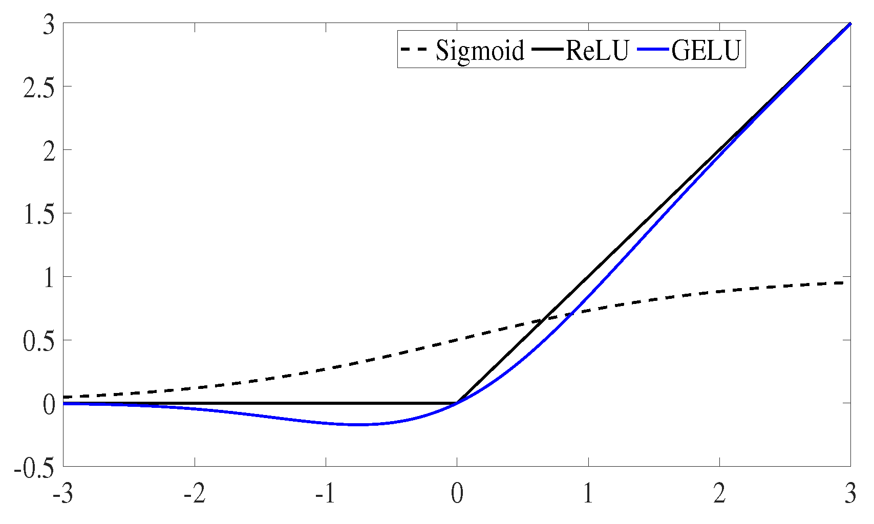GELU example

This is assembled into the MLP result of size $[C_{\text{embed}},T]$. Like in the self-attention + projection section, we add the result of the MLP to its input, element-wise to produce the MLP residual.

This marks the end of the transformer block and the output is ready to be passed to the next block.

Output

Finally, at the end of all the transformer blocks, we perform one final softmax, which helps convert the output into probabilities.

Multi-class Probabilities

See also: multi-class classification

The softmax function allows us to map $k$ real numbers $z_i=w_c^T{x}_i$ to probabilities.

$P(y|z_1,z_2,\dots ,z_k)=\frac{\exp (z_y)}{{\sum }_{c=1}^k\exp (z_c))}$

The alternative ‘harder’ version to softmax is the argmax function which simply finds the maximum value, sets it to 1.0, and assigns 0.0 to all other values.

In contrast, the softmax operation serves as a “softer” version of that. Due to the exponentiation involved in softmax, the largest value is emphasized and pushed towards 1.0, while still maintaining a probability distribution over all input values. This allows for a more nuanced representation that captures not only the most likely option but also the relative likelihood of other options.

Link to original

We then take this $[C_{\text{embed}},T]$ output block and do a final matrix multiply with another set of learned weights called the language modelling head weights (LM weights) which is a $[n_{\text{vocab}},C_{\text{embed}}]$ matrix.

This produces the logits of size $[n_{\text{vocab}},T]$. The name “logits” comes from “log-odds,” i.e., the logarithm of the odds of each token. Finally, we softmax this again to exponentiate the log-odds to normal odds/probabilities.

Now, for each column, we have a probability the model assigns to each word in the vocabulary. Then, we can ‘decode’ the final probability back into a token. For example if we’ve supplied six tokens into the model, we’ll use the output probabilities of the 6th column.

We do this by “sampling from the distribution.” That is, we randomly choose a token, weighted by its probability. For example, a token with a probability of 0.9 will be chosen 90% of the time.

We can also control the “smoothness” of the distribution by using a temperature parameter. A higher temperature will make the distribution more uniform, and a lower temperature will make it more concentrated on the highest probability tokens.