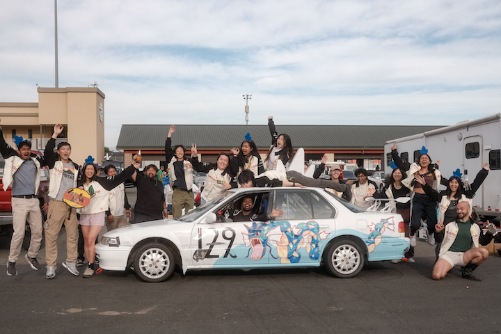
I drive a manual 1992 Honda Accord in 24 Hours of Lemons as a part of our team Magicarp Motors.
A big part of the fun was to make our spectator experience as good as, if not better than, the F1 viewing experience. We wanted people to be able to come to the race, really feel immersed in the intensity of it. We wanted people to see the intense passes, the g-forces on each turn and braking zone, and hear the engine hum and tires squeal.
Part of that was making sure we could get live and accurate video and telemetry streams overlaid in a way so that people from the paddock and those at home could watch.
Though the car itself is something we worked on over the course of many months, this telemetry and live streaming setup was built by Shihao1 and I over the course of about a week in late March before our Sonoma race.
Reading values
The main commercial options (RaceChrono, Harry’s Lap Timer) get your phone GPS (which is normally only accurate to ~10m) and maybe an OBD-II connection which lets you tap values from the ECU directly. Unfortunately for us, the Honda Accord was made in 1992 which predates the OBD-II protocol that most modern telemetry and diagnostics tools.
Shihao then had the brilliant idea of just manually tapping wires for values we cared about.
His post goes into more details about this process but the tldr; is that there were 3 main classes of signals from the car we cared about:
- 12V analog (brake indicator, battery voltage)
- 5V analog (throttle position, engine coolant temp, manifold absolute pressure)
- 12V square wave (RPM, vehicle speed sensor)
The analog values were read via an onboard Arduino. We also wanted GPS, accelerometer, and gyroscope readings which the ECU did not provide so we bought a Racebox Micro for those.
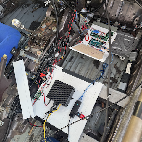
All of this was fed into an onboard Jetson Nano that we used to run a custom built telemetry server which ingested both the Arduino and Racebox data feeds.
Frequency measurement
One really neat thing that I didn’t think about until we started doing live driveway tests was how to interpolate rapidly changing values.
The Arduino firmware originally uses a 16-slot ring-buffer of micros() timestamp of when the last pulses happened.
Square wave reading
    ┌─┐ ┌─┐ ┌─┐ ┌─┐ ┌─┐ ┌─┐         ...
  ──┘ └─┘ └─┘ └─┘ └─┘ └─┘ └─────────────  time →
    ↑   ↑   ↑   ↑   ↑   ↑
    recordPulse() → micros() stamped each rising edge

Ring-buffer
					   head ─┐ (next write)
 idx:  0    1    2    3   …  │ … 15
	  ┌────┬────┬────┬────┬─▼──┬────┐
	  │ t₀ │ t₁ │ t₂ │ t₃ │ .. │ t₁₅│   (timestamps in µs)
	  └────┴────┴────┴────┴────┴────┘
		↑oldest          newest↑
However, the problem was that this approach would overestimate in rapid deceleration (important for correctly reporting RPMs in intense braking conditions!).
Say the engine is at 5000 RPM and drops to 1000 RPM. The last five pulses in the ring buffer came in at 100, 102, 104, 106, and 108ms. It’s now 150ms and no new pulses have arrived.
The naive approach — what I’m calling pulse-only frequency — looks at the oldest and newest pulse in the buffer: 5 pulses over 8ms = 625 Hz. This reflects what the engine was doing, not what it’s doing now. During deceleration it massively overestimates because all those pulses arrived when RPM was still high, and the 42ms gap since the last pulse is invisible.
Hz
100 ┤█  █  █  ░
    │█  █  █  ░  ░
 80 ┤█  █  █  █  ░  ░
    │█  █  █  █  █  ░  ░
 60 ┤█  █  █  █  █  █  ░  ░
    │█  █  █  █  █  █  ░  ░  ░
 40 ┤█  █  █  █  █  █  █  ░  ░  ░
    │█  █  █  █  █  █  █  █  ░  ░
 20 ┤█  █  █  █  █  █  █  █  █  █
    │█  █  █  █  █  █  █  █  █  █
  0 ┼──────────────────────────────► t
     └ steady ┘ ↑ deceleration begins

█ true frequency      ░ overestimate
A better measure is frequency-including-gap-to-now: use the span from the oldest pulse to the current time. That gives 5 pulses over 50ms = 100 Hz. The growing gap since the last pulse pulls the estimate down as the engine slows.
real period keeps growing as we decelerate → →
edges:  ●──●──●───●────●──────●         ┊now
	  t₀ t₁ t₂  t₃   t₄     t₅          ┊
	  |←─── span_pulses ───→|           ┊
							|←── gap ──→|
	  |←───────── span_to_now ─────────→|

pulse-only = (count-1) / (t_newest - t_oldest)
gap-to-now = count / (t_now - t_oldest)
We take the minimum of the two: min(625, 100) = 100. This gives the right answer in every regime. During steady state, both methods agree. During deceleration, the gap-to-now method is lower (correct). During acceleration, the pulse-only method is lower (also correct, you don’t want to overcount based on future expectations). Without this, the tach hangs at the old RPM reading during engine braking until enough new slow pulses fill the ring buffer.
Telemetry server
The Jetson has 4GB of RAM and limited storage. My initial prototype just shoved all the data in memory but on a long test drive it OOM’d at ~16 million entries. Afraid of losing data again, we built a very simple durable storage system for the entries that is basically a log-structured store.
			append(tick)
				 │
				 ▼
┌──────────── log-structured store (source of truth) ──────────┐
│ .append → write(2) every write, fsync(2) every 100 writes    │
│     │                                                        │
│     ├──► live view:  emit "entry" → SSE /stream → UI         │
│     │                                                        │
│     └──► appended to active segment on disk  /data/wal/      │
│           ┌────────────────────────────────────────────┐     │
│           │ wal.000001.log  sealed   #range:1–5000     │     │
│           │ wal.000002.log  sealed   #range:5001–10000 │     │
│           │ wal.000003.log  ACTIVE   (appending)       │     │
│           └────────────────────────────────────────────┘     │
└──────────────────────────────────────────────────────────────┘

history view:  getTicksInRange(seqRange) → replay segments
                 (#range footers skip non-overlapping segments)
Durability is a tradeoff with fsync(2).
writeSync= thewrite(2)syscall → bytes land in the OS page cache. Cheap. Survives a process crash (kernel keeps the cache) but not a power loss.fsync= force the page cache to the physical device. Expensive (a real flush + barrier). This is the only thing that survives power loss.
Most normal systems bound fsync frequency to around ~1 fsync per second (which bounds power-loss dataloss to a ~1 second window). Too much fsync reduces your IO throughput significantly and also increases flash wear (which matters for our system which runs off an SD card).2
Calculations
Lap detection
The main thing I wanted was automated lap detection logic so race engineers didn’t need to manually track it.
I manually ended up mapping track data by making a track annotation tool that outputted the polyline for the track. This allowed me to get granular with labelling turns on Sonoma (and also make a little test track around the block which we could drive around to test).
A problem then became how we would project the actual car position onto this polyline. Turns out we can just use linear algebra3 and project the GPS point to the nearest segment via a dot product!
                     ● GPS reading
                     ┊
                     ┊ ⟂  perpendicular — keep the nearest segment
                     ▼
•╮              A          B
 ╰•╮           ╭•────X─────•╮
   ╰•╮       ╭•╯            ╰•╮
     ╰•─────•╯                ╰•── … ──►

X = A + t·(B−A)                                the projection itself

t = clamp(0, (● − A)·(B − A) / |B−A|², 1)      fraction along A→B

progress = (segDist[A] + t·|AB|) / totalDist   arc-length, 0..1


- • are the polyline points of the track centerline
- A, B are the endpoints of the cloest segment in the track
- X is the projection of ● onto the track
- segDist is mapping of • to cumulative distance
- totalDist is the sum of all the distances across the points
A finish line crossing is detected when progress drops from above 0.85 to below 0.15 (the wraparound). First lap is automatically flagged as an out lap; stopping a session flags the current lap as an in lap.
Pace deltas
A pace delta tells you how much time you are ahead or behind of your best lap at your current position on the lap.
Given that we just did all that ‘track progress’ work to figure out lap detection, we can actually compute these deltas quite easily.
We do this by first building a reference curve from the best lap. For each GPS point, store its progress and elapsed time. This gives a monotonically increasing curve that represents “how long the best lap took to reach each point on track.” To query, take the current GPS position, project it to get progress (say 0.42). If the best lap reached 0.42 at 28.3s4 and you’re at 27.8s, delta = −0.5s.
elapsed

28s ┤                     █
    │                  █  █
    │                  █  █
    │                  █  █
    │               █  █  █
    │            █  █  █  █
14s ┤┄┄┄┄┄┄┄┄┄█  █  █  █  █
    │         █  █  █  █  █
    │         █  █  █  █  █
    │      █  █  █  █  █  █
    │   █  █  █  █  █  █  █
 0s ┤█  █  █  █  █  █  █  █
    └─────────┴──────────────► progress
     0       0.42           1

              ╵
        query this progress
You can even get a full ‘delta graph’ mapping delta to track position by subtracting the two reference curves:
 Δ = this lap − best lap

+Δ ┤      █  █
   │   █  █  █  █
 0 ┼──────────────────────────────────────► progress
   │                  █  █  █  █  █  █
   │                     █  █  █
−Δ ┤                        █
   0                                       1

+Δ = behind best lap
−Δ = ahead
 0 = best lap (reference)
Interestingly though, my approach here differs from my understanding of what industry-standard is. Most systems integrate wheel speed into distance: , reset to zero each time you cross start/finish.
Then, the error in the final accumulated distance (what we’ll call ‘drift error’) is then . Integrating noise is a random walk so its variance grows linearly with each sample: the error’s standard deviation grows with .
e_d based on VSS

+ ┤                            ░░░░░░
  │                    ░░░░░░░░░░░░░░
  │             ░░░░░░░░░░░░░░░░░░░░░
  │        ░░░░░░░░░░░░░░░░░░░░░░░░░░
  │     █░█░░░░░░░░░░░░░░░░░░░░░░░░░░
  │  ░░█░█░█░░░░░░░░░░░░░░░░░░░░░░░░░
  │ ░░█░░░░░█░░░█░░░░░░░░░░░░░░░░░░░░
0 ┤█░█░░░░░░░█░█░█░░░░░░░░░█░█░░░░░░░
  │ █░░░░░░░░░█░░░█░░░░░█░█░█░█░░░░░░
  │  ░░░░░░░░░░░░░░█░░░█░█░░░░░█░░░░░
  │     ░░░░░░░░░░░░█░█░░░░░░░░░█░░░░
  │        ░░░░░░░░░░█░░░░░░░░░░░█░█░
  │             ░░░░░░░░░░░░░░░░░░█░█
  │                    ░░░░░░░░░░░░░░
− ┤                            ░░░░░░
  └──────────────────────────────────► t

 ░  ±σ√t envelope (typical spread)    █  one actual run (random walk)
Reading position directly on the other hand never integrates, so the error just sits constant at the GPS noise floor the same at lap end as at lap start.
e_d based on GPS

+ ┤░█░█░░░█░░░░░░░█░░░░░░░█░█░░░░░░░█
0 ┤█░█░█░█░█░█░█░█░█░█░█░█░█░█░█░█░█░
− ┤░░░░░█░░░█░█░█░░░█░█░█░░░░░█░█░█░░
  └──────────────────────────────────► t

 ░  ±σ_x band (constant)             █  one actual run
Streaming
Finally, the last part is how we eventually get the data off the Jetson and back to our ground station.
Overlay network
Our Jetson itself connects to a 5G modem with a SIM card that we bolted to the roof of the car. This is connected to the same Tailscale network as my laptop which lets both devices see each other as ‘on the same network.‘
Video Streaming
We have two separate webcams, one for the dash view and the other for the driver view. As we used pretty cheap webcams, they didn’t support native H.264 capture. Fortunately for us though, we have a Jetson Nano which we took full advantage of to encode the video onboard before sending it across the wire.
Our captures happening in MJPEG and we had a GStreamer pipeline that went through jpegdec → nvvidconv → nvv412h264enc → MPEG-TS → SRT.
One thing that we had lots of trouble tweaking was what the optimal encoding + SRT settings were for our use case of low-latency unreliable streaming (as the reception on the track was definitely spotty).
We saw some pretty bad ‘frame bleed’ where reference frames were dropped but subsequent motion deltas arrived and thus smeared the incorrect anchor frames, etc. If anyone reading this has experience working in video encoding in these environments I’d love to hear from you!
Fin
This is not to say our telemetry setup is anywhere near done. There’s still a lot of data around the actual physics of tire traction I’d like to get setup, along with a lot more tapping of non-ECU systems like brake temperatures, tire temperatures, gearbox position, etc.
But this is also not the end of our racing story either! Our team is planning on racing again at 24h of Lemons Buttonwillow in September and hopefully we will have some interesting follow up work to write about here as well.
Thank you to Shihao for hacking on this with me.
You can find the code for our telemetry setup over on our team’s GitHub repository.
If you find this kind of stuff fascinating and want to support a group of friends working on this sort of thing, please consider sponsoring or donating to our team, it would really mean a lot and would help us meaningfully make this accessible to all of our team members :)
Footnotes
-
Shihao talks more about the hardware side of the telemetry stack on his blog. ↩
-
Writing this in hindsight, the 4s dataloss window here (100 write window / 25 writes per second) is quite large. I might go change that to be 0.5 - 1s! ↩
-
This is kinda leaving out the fact that we are treating latitude/longitude as plain
(x,y)coordinates on a flat plane but the Earth believe it or not is a sphere. Technically to be accurate we should not be using the Euclidean norm but rather the Haversine distance which computes great-circle distance (i.e. the ‘surface’ distance on a sphere). ↩ -
The best lap won’t have a point at exactly 0.42, so linearly interpolate between the two nearest. ↩